How to Fix Excel Errors: #REF!, #VALUE!, #NAME? and More
Updated 2026-10-25 · Free · Works in your browser
Quick answer
Excel errors tell you exactly what is wrong: #REF! means a formula points at a deleted cell, #VALUE! means a wrong data type (usually text where a number is expected), #NAME? means Excel does not recognize a function or range name, and #DIV/0! means division by zero or blank. Click the error cell, read the formula bar, and fix the reference, the data, or the spelling.
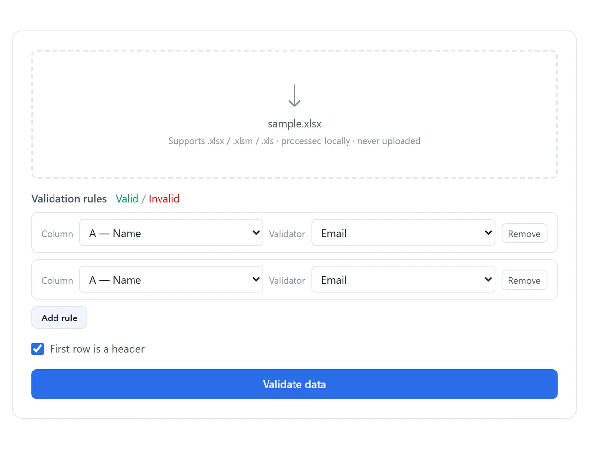
Skip the reading — jump straight to the free tool: Validate Excel Data →
The Error Decoder
| Error | What it means | First thing to check |
|---|---|---|
| #REF! | A formula points at a cell, range or sheet that no longer exists | What was deleted or moved recently |
| #VALUE! | Wrong ingredient type — usually text where a number is expected | Hidden spaces or text-formatted numbers in the inputs |
| #NAME? | Excel does not recognize a function or named range | Spelling, missing quotes around text, unsupported function |
| #DIV/0! | Dividing by zero or by an empty cell | The divisor cell |
| #N/A | A lookup found nothing | Whether the lookup value really exists, with matching type |
| #NUM! | Invalid numeric result — too large, or impossible like SQRT(-1) | The math itself |
| #NULL! | Two ranges were asked to intersect but don’t (space operator) | A stray space between ranges in the formula |
| ##### | Not an error: column too narrow, or a negative date/time | Widen the column; check the date value |
| Circular reference | A formula depends on its own result | The cell named in Excel’s status bar warning |
Errors cascade: any formula that references an error cell shows an error too. When a sheet lights up, fix the upstream cells first and the rest often clears on its own.
#REF! — The Formula Points at Something That No Longer Exists
- Just happened? Press Ctrl+Z immediately — undo restores the deleted rows, columns or sheet and the reference with it.
- Too late for undo: press Ctrl+H and Find what: #REF! — Excel finds every broken formula at once, so you can re-point each reference by hand.
- If a whole named range was deleted, rebuild it under Formulas ▸ Name Manager and the formulas heal themselves.
- For links to other workbooks that moved: Data ▸ Queries & Connections ▸ Edit Links and repoint to the new file location.
If #REF! appeared right after deleting rows or columns, do not save — close without saving and redo the deletion with the formulas in mind. A saved #REF! cannot be auto-restored.
#VALUE! — Right Formula, Wrong Ingredients
The formula is syntactically fine but is fed something it cannot digest: numbers stored as text (the green-triangle cells), invisible trailing spaces or non-breaking spaces pasted from the web, or dates that are actually text.
- Numbers stored as text: select the column ▸ click the warning icon ▸ Convert to Number — or bulk-fix the whole file in one pass with a converter.
- Hidden spaces: wrap the input in TRIM(), or strip trailing/non-breaking spaces from the entire sheet at once.
- Text dates: re-enter them in a real date format, or convert the column so date arithmetic works.
#NAME? — Excel Doesn’t Recognize That Word
- Typo in the function name: VLOKUP, SUMIFs with wrong casing of arguments typed from memory — check the spelling against the official syntax.
- Text typed without quotes: =IF(A1=yes,…) must be =IF(A1="yes",…).
- A named range that was renamed or deleted — verify under Formulas ▸ Name Manager.
- A function your Excel version doesn’t have: XLOOKUP, LET, FILTER and other dynamic-array functions show #NAME? in Excel 2019 and older. Replace them with INDEX/MATCH-style equivalents, or open the file in a newer Excel.
#DIV/0! and #N/A — The Divide-and-Lookup Twins
- #DIV/0!: the divisor is zero or empty. Common with AVERAGE of an empty range or a percentage whose base is blank. Guard the formula:
- #N/A: VLOOKUP/XLOOKUP/MATCH found nothing. Either the value truly is absent, or it exists with a different type (number vs text) or trailing spaces — the two most common false alarms.
- When “nothing found” is a legitimate outcome, present it cleanly instead of as an error:
=IFERROR(A2/B2, "")        // blank instead of #DIV/0!
=IFNA(VLOOKUP(A2, D:E, 2, FALSE), "not found")   // text instead of #N/A
IFERROR hides the symptom, not the cause. Fix the underlying data first; use IFERROR only for cases where “not found / not applicable” is a real answer, not a surprise.
#####, #NUM!, #NULL! and Circular References
- ##### : the column is too narrow for the number — widen it. If it stays after widening, the value is a negative date or time, which Excel cannot display.
- #NUM!: the math is impossible or out of range — SQRT(-1), or a result beyond Excel’s limits. Check the inputs.
- #NULL!: a space between two ranges asked for an intersection that doesn’t exist, e.g. =SUM(A1:A5 C1:C5). Replace the space with a comma or colon.
- Circular reference: the formula’s own cell is part of its input. Excel names the cell in the status bar and in Formulas ▸ Error Checking ▸ Circular References. Move the formula or fix the logic — enable iterative calculation only if you intentionally designed a loop.
Stop Errors Before They Spread
- Validate at the door: restrict inputs to the type each column expects — numbers as numbers, dates as dates — so #VALUE! never gets raw material.
- Look up function syntax before writing, not after the error.
- Keep a clean copy: a version snapshot before big edits turns “everything shows #REF!” from a disaster into an undo.
Tools Used in This Guide
Frequently Asked Questions
How do I find all errors in a large sheet at once?
Press Ctrl+G ▸ Special ▸ Formulas ▸ tick only Errors ▸ OK. Excel selects every error cell — fix the ones other formulas depend on first, and the rest usually clears.
Does IFERROR actually fix the error?
No — it masks the display. The underlying problem is still there. Fix the reference or the data first, then use IFERROR only to present legitimate “empty/not found” outcomes.
Why did working formulas turn into #NAME? on another computer?
The other Excel is older and lacks the function — XLOOKUP, LET, FILTER and similar need Excel 2021 or Microsoft 365. Rewrite with INDEX/MATCH-era functions for compatibility.
VLOOKUP returns #N/A even though the value is clearly there — why?
Type mismatch or hidden spaces: a number looked up against text, or trailing spaces in one side. Convert both sides to the same type and trim the spaces, and the match appears.
Are Excel errors contagious?
Yes. Any formula referencing an error cell errors as well, so one bad cell can paint a whole sheet red. Always fix the most upstream error first.
Related Guides
Ready to try it on your own file?
Open Validate Excel Data — It's Free